Implementing and Benchmarking Classic Algorithms
Stable matching, greedy against dynamic programming, and the closest pair of points. Each one implemented, then benchmarked against the alternatives instead of trusting the complexity class on paper.
What this is
Coursework for IFT 2125, Introduction to Algorithms at Université de Montréal. One assignment, three classic problems, each with a theory half and an implementation half. The interesting part is the second one: every algorithm had to run against a benchmark harness and be timed on the same inputs as its rivals.
That turns an asymptotic bound into something you can be wrong about. Twice here the measurement disagreed with the intuition, which is the whole reason for taking the numbers.
How correctness was checked
Timing a wrong answer is worthless, so the harness carries known optimal solutions and verifies each result within a tolerance before any speed comparison counts. For stable matching it goes further and scores what fraction of couple pairs are actually stable, so a near miss is visible rather than being a pass or fail.
The three problems
Stable matching
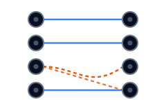
Pair everyone on one side with someone on the other so that no two people would both rather swap.
- Gale-Shapley built twice: one pre-sorts every preference list with a single
argsortand advances a pointer per proposer, the other keeps an n by n already-proposed matrix and rescans for the best remaining option every round - Both hold a partner array plus a worklist of free proposers, pushing anyone who gets rejected back onto it
- Three baselines for contrast: best still-free partner in index order, a symmetric variant that sorts all n squared edges by the sum of both sides' scores, and a trivial one pairing index to index
- Every variant ends by calling the harness stability score, so all five are judged the same way. Gale-Shapley is O(n2) in the worst case, since each proposer can work through the whole list once
Greedy against dynamic programming
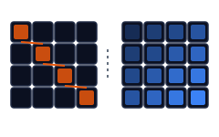
The same matching problem again, now with a structure that makes an exact solution reachable.
- The constraint is that edges may not cross: an edge to a later row must not land on an earlier column, tested against every edge already chosen
- The greedy sorts all n by m edges by weight and takes one when both endpoints are free and nothing already chosen crosses it, so each candidate rescans the matching so far
- The dynamic program fills an (n+1) by (m+1) table with
max(up, left, diagonal + X[i][j]), the same shape as a weighted longest common subsequence - A traceback from the bottom-right corner rebuilds which edges were actually taken. The table is O(nm) to fill; the greedy pays a sort plus a crossing rescan per candidate edge
Closest pair of points
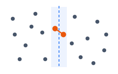
Find the two nearest points in a plane, faster than comparing all pairs.
- Sorted by x and by y once up front, then the recursion splits x at the midpoint and partitions the y-ordered list against that same midpoint, so y-order survives without ever re-sorting
- The strip keeps points within the current best distance of the dividing line, and the inner loop compares each one against only the next seven. That constant of seven is the answer to the theory question the code is built around: a packing argument bounds how many points can sit inside the strip without already being closer than the best distance found
- The second build sorts by x once but re-sorts the corridor by y inside every recursive call, which is the whole difference between the two curves below
- It also works in squared distances, keeping the square root out of the inner loop, which turned out not to be enough to save it
The measurements
Re-run for this page on a Ryzen 7 7700 under Python 3.12, averaged over repeated trials at each size: 64 runs at the smallest n falling to 2 at the largest, which is why the bars widen on the right.
Stability of the result
Share of couple pairs that come out stable. Bars are two standard deviations; Gale-Shapley has none, returning a perfectly stable matching on every single run.
Show the numbers
| n=20 | n=40 | n=80 | n=160 | n=320 | n=640 | |
|---|---|---|---|---|---|---|
| Gale-Shapley | 1.000 | 1.000 | 1.000 | 1.000 | 1.000 | 1.000 |
| Greedy (best pair) | 0.913 | 0.938 | 0.961 | 0.975 | 0.987 | 0.992 |
| Greedy (trivial) | 0.544 | 0.559 | 0.559 | 0.561 | 0.550 | 0.548 |
Greedy against dynamic programming
Same instances, both measures. The exact solution wins on speed and on score at every size, which is not the trade the textbook sets up.
Show the numbers
| n=32 | n=64 | n=128 | n=256 | n=512 | n=1024 | |
|---|---|---|---|---|---|---|
| Greedy | 310 µs / 870 | 1.4 ms / 1,490 | 7.0 ms / 3,199 | 30.2 ms / 5,867 | 201.5 ms / 9,276 | 967.0 ms / 11,785 |
| Dynamic programming | 290 µs / 1,660 | 1.1 ms / 3,308 | 4.2 ms / 6,885 | 16.4 ms / 13,889 | 71.0 ms / 27,796 | 299.5 ms / 55,858 |
Cost of sorting in the wrong place
Closest pair, same inputs. Measured growth from 10⁴ to 10⁵ is 13.9 times for a tenfold rise in n, which is what n log n predicts.
Show the numbers
| n=10 | n=100 | n=1,000 | n=10⁴ | n=10⁵ | |
|---|---|---|---|---|---|
| Sort once, then divide | 9 µs | 132 µs | 2.2 ms | 30.0 ms | 418.8 ms |
| Divide, then sort | 18 µs | 251 µs | 3.7 ms | 59.5 ms | 982.7 ms |
What the numbers said
First, what the timing does not show
The stability chart comes with a caveat found by reading the harness rather than its output. Scoring a matching compares every pair of couples, so it costs order n squared, and it runs inside the region being timed. The trivial baseline builds its answer in linear time yet still costs 107 ms at n = 640, against 102 ms for a full Gale-Shapley run. Almost all of both numbers is the scoring, not the algorithm.
So the honest reading is narrow. The stability comparison stands, because that axis is uncontaminated. The gap between the two Gale-Shapley builds stands, because it is far larger than the shared floor. Any claim that one matching algorithm is faster than another would not, on this harness. Noticing that a benchmark is partly measuring itself is the part worth keeping.
The implementation beat the algorithm
Both Gale-Shapley builds are O(n2) and return identical matchings, yet one runs 3.8 times slower at n = 640: 388 ms against 102 ms. The only difference is one argsort per preference list against an O(n) rescan on every proposal. Same asymptotics, same output, and the constant decided it.
Greedy lost on both axes
The expected trade is faster but worse. Against an O(nm) dynamic program the greedy was worse and slower: 967 ms to 300 ms at n = 1024, scoring 11,785 against 55,858. Sorting every edge and rescanning the matching for crossings costs more than filling the table, and taking heavy edges first blocks the ordering the exact solution exploits.
A flat sweep that was really a bug
Sweeping the brute-force cutoff on the first closest-pair build changed nothing, which looked like a tidy null result. Reading the code explained it: that build hardcodes its base case at three points and never reads the parameter. On the build that does read it, the same sweep spans 2.3 times, 58 ms to 133 ms, with a clear optimum at 24.
An optimisation that did not pay
The slower closest-pair build is also the one that avoids a square root, comparing squared distances in its inner loop while the faster build calls a real distance function. It still loses by 2.3 times, because re-sorting the corridor on every recursive call costs far more than the square roots it saves. Cheaper arithmetic inside a worse traversal is not a saving.